info
Liquefaction Triggering Methods (All computed by default)
SPT-Based Procedures
• NCEER Consensus Procedure (Youd et al., 2001)
• Boulanger & Idriss (2014) Updated Procedure CPT-Based Procedures
• Robertson & Wride (1998) with Robertson (2009) update
• Boulanger & Idriss (2014) CPT Procedure Both methods are computed automatically for each test type. Excel export includes separate sheets for each method.
Select unit system for calculations and Excel report display.
settings_input_component
Seismic Parameters Input
Default: 760 m/s
Site Class: Class -
We automatically compute Mw for 475 yr (DBE, 10% in 50) and
2475 yr (MCE, 2% in 50).
Mw input for liquefaction will auto-fill from the 2475-yr mean Mw when available.
check_circle
USGS Data Retrieved
PGAM:- g
SDS:-
SD1:-
TL:- sec
Model:-
Vs30:- m/s
Site Class:-
475 yr (DBE)
Mean Mw:-
Mean r:- km
Mean ε0:-
2475 yr (MCE)
Mean Mw:-
Mean r:- km
Mean ε0:-
info
format_list_numbered
Drilling Data Input
(m)
(m)
(m)
(m)
datasetInput DIGGS Files
DIGGS XML map is independent from the USGS workflow. Select boreholes/tests and import into the tables.
Total0CPT0SPT0
None selected
Search public historic boreholes around a point. (This does not auto-download DIGGS yet; it provides links for manual download/import.)
Tip: pan/zoom the map. When you zoom in, markers resolve to exact borehole locations.
layers
Stratigraphic and Groundwater Level Settings
(m)
Multiple levels separated by commas
No
Soil Type
Drainage
Depth (m)
γt (kN/m³)
Illustrate
Analysis above
Sand Surge Analysis
map
Import from DIGGS Map
Load boreholes from DIGGS XML and click a point to import soil type and unit weight into the table above. Use the same workflow as the Liquefaction page.
Boreholes:0
Click "Load DIGGS map" to show map
timeline
Excavation Order and Water Level Input
Enter water levels for each excavation stage. Use the initial groundwater level if not specified.
Excavation Stage
Depth (m)
Under Development: this module is not finalized yet.
settings_input_component
Input Parameters
Design Code & Standards
1. Toe Stability / Kick-out
Standard: USACE EM 1110-2-2504 (or FHWA GEC 4)
Rationale: Both standards use the same logic for calculating "passive earth pressure resistance against kick-out" (Free Earth Support Method).
Program Setting: Fixed FS ≥ 1.5
2. Basal Heave
Standard: NAVFAC DM 7.02
Rationale: This is the most classic reference for handling heave in soft clay. When American engineers discuss Heave, they refer to NAVFAC.
Program Setting: Fixed FS ≥ 1.5
3. Piping/Boiling
Standard: USACE / FHWA General Standards
Program Setting: Fixed FS ≥ 1.5
(m)
(m)
(m)
(kN·m/m)
-
settings
Analysis Conditions
dynamic_feed
Surcharge / External Loads
SUC: uniform surcharge converted to equivalent lateral pressure increment. SUB: depth-dependent lateral pressure from Boussinesq records.
(kPa)
(kPa)
SUB Records
No
Z (m)
A (m)
B (m)
Q (kPa)
Action
image
Illustrative Diagrams
layers
Stratigraphic and Groundwater Level Settings
(m)
(m)
Layer Parameters
Layered Water Level Input Mode
No
Layer Code
Drainage
Depth (m)
γt (kN/m³)
c' (kPa)
φ' (deg.)
Su/σv'
SPT-N
Dw,exc (GL-m)
Dw,ret (GL-m)
Seepage Mode
map
Import from DIGGS Map
Load boreholes from DIGGS XML and click a point to import soil type and unit weight into the table above.
Boreholes:0
Click "Load DIGGS map" to show map
bar_chart
Interactive Profile
Under Development: this module is not finalized yet.
settings_input_component
Input Parameters
(m)
(m)
-
settings
Analysis Conditions
image
Illustrative Diagrams
Cantilever Wall Analysis
layers
Geological Strata and Groundwater Pressure Settings
(m)
(m)
No
Soil Type
Layer Type
Depth (m)
γt (kN/m³)
c' (kPa)
φ' (deg.)
Su (kPa)
SPT-N
Dw,exc (GL-m)
Dw,ret (GL-m)
Seepage Mode
bar_chart
Interactive Profile
Shallow Foundation
straighten
Unit System
Select unit system for inputs and results.
straighten
Foundation Geometry
Methods mainly differ in the bearing capacity factors (especially \(N_\gamma\)) and which correction factors are applied.
Long-term load bearing safety factor=
Short-term load bearing safety factor=
Ultimate limit state bearing safety factor=
vertical_align_center
Service Loads (kN, kN·m)
Type
Vx
Vy
Pz
Mx
My
D
L
W
E
image
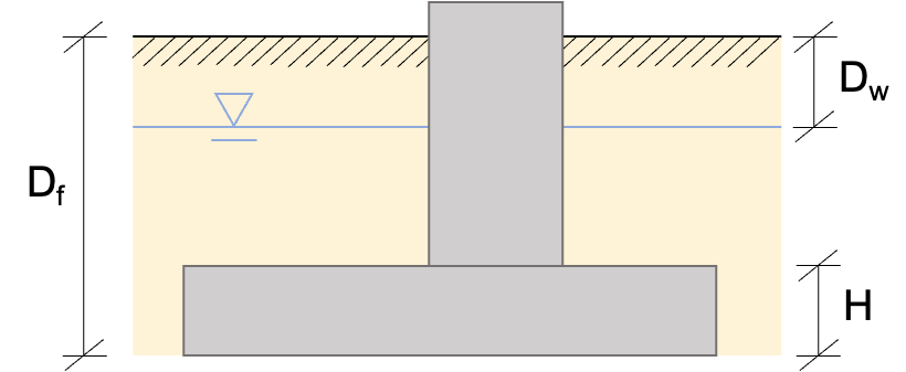
Schematic
Side View
Place shallow1.png in static/images/
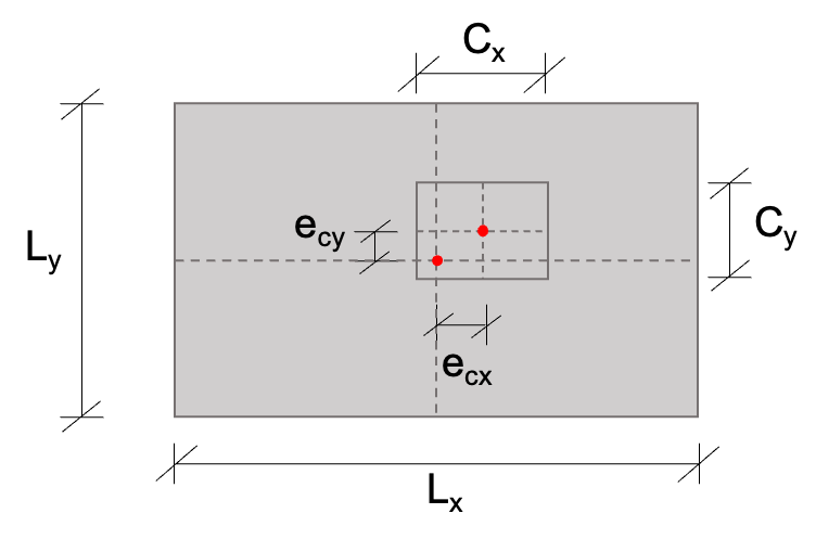
Plan View (Top View)
Place shallow2.png in static/images/
layers
Stratigraphic Settings
ztop (m)
zbot (m)
γt (kN/m³)
Soil Class
Drainage
Su (kPa)
c′ (kPa)
φ′ (°)
Load boreholes from DIGGS XML and click/select a borehole to import soil layers into the table above.
0
Click "Load DIGGS map" to show map
Pile Foundation Analysis
Under Development
Pile Foundation module coming soon...
Retaining Wall Analysis
Under Development
Retaining Wall module coming soon...
Calculation points illustration×
Image loading failed
Please place the image at: static/images/calculation_points.png
SPT Depth BottomSPT Mid-point
Site Class Reference (ASCE 7 / NEHRP)×
Class A — Hard Rock (> 1,500 m/s)
Class B — Rock (760 – 1,500 m/s)
Class BC — Soft Rock / USGS Reference (760 m/s)
Class C — Very Dense Soil / Soft Rock (360 – 760 m/s)
Class D — Stiff Soil (180 – 360 m/s) [Common Default]
Class E — Soft Clay Soil (< 180 m/s) [High Risk]
Class F — Special Soils (Requires Site Response Analysis)
Processing…
Uploading and processing XML. Please wait.
Liquefaction Analysis Summary×
Factor of Safety (FS) Analysis Results
About DIGGS×
DIGGS is an XML/GML-based data transfer standard for geotechnical and geoenvironmental information.
Use comma-separated groundwater levels for each impermeable interface (U layer), for example:
2, 4.5, 8.
Order must be from top to bottom interface. If fewer values are provided than interfaces, the last value is reused.
Units follow the selected unit system: m in Metric, ft in Imperial.
Water Pressure Analysis Mode
×
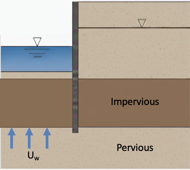
Static Water Pressure (No Seepage)
The groundwater levels on both the retaining side and excavation side exhibit static water pressure distribution, without considering the effects caused by water pressure differences on both sides of the retaining wall.
When using non-watertight retaining walls (steel rail piles, steel sections, soldier piles), this mode is generally applicable when the original formation exhibits static water pressure distribution. Since (after dewatering on the excavation side) the water levels on both sides of the retaining wall are the same, please enter the same value for the retaining side groundwater level Dw,ret and the excavation side groundwater level Dw,exc.
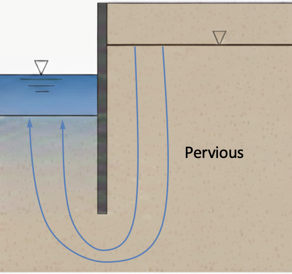
Triangular Water Pressure (With Seepage)
The groundwater levels on the retaining side and excavation side are different, causing seepage due to the water pressure difference at the bottom of the retaining wall. This mode is applicable to watertight retaining walls (diaphragm walls, sheet piles) in thick permeable formations (sand, gravel, cobble), without clay interlayers.
After horizontal seepage at the wall bottom, CATii automatically calculates the water pressure using the following formula:
Layered Water Level Input
This mode is applicable to various formation conditions. For formations with alternating sand and clay layers, it is recommended to prioritize this mode. After inputting the water levels of each layer and seepage mode according to the construction dewatering conditions, CATii can automatically calculate vertical seepage and horizontal seepage at the wall bottom. For input methods, please refer to the Layered Water Level Input Mode description.
Service Loads
×
Service loads represent the unfactored working load combinations used to evaluate foundation performance under normal operating conditions. These combinations include permanent loads (D), live loads (L), wind loads (W), and seismic loads (E), combined according to service-level requirements.
The resulting forces and moments are used to assess eccentricity effects, contact area reduction, and allowable bearing capacity under working stress conditions.
Seepage and Sand Boil Safety Factor Formulations
×
This platform evaluates seepage-induced instability using classical hydraulic gradient and uplift stability concepts widely adopted in U.S. levee and dam engineering practice.
The formulations implemented here are based on:
Terzaghi's critical hydraulic gradient theory
Lane's weighted creep theory
U.S. Army Corps of Engineers (USACE) seepage design manuals
These methods are commonly used for preliminary assessment of uplift, heave, and piping risk in earth structures.
This equation compares the total vertical soil weight above the potential uplift plane with the upward hydraulic force generated by excess pore water pressure.
If \( FS_u < 1.0 \), uplift failure may occur. Design guidelines typically require \( FS_u \ge 1.2 \).
This expression is derived from the ratio \( FS = i_{cr} / i_{exit} \), where \( i_{cr} = \gamma'/\gamma_w \) is the critical hydraulic gradient (Terzaghi) and \( i_{exit} = \Delta H/(2D) \) is the exit gradient at the seepage face.
Design guidance typically requires \( FS_{p1} \ge 1.5 \).
References: Terzaghi (1943), Theoretical Soil Mechanics; USACE EM 1110-2-1901
This formulation reflects seepage path length considerations based on classical creep theory developed by Lane (1935). It represents a simplified expression of weighted seepage path resistance.
References: Lane (1935), "Security from Under-Seepage – Masonry Dams on Earth Foundations"; USACE EM 1110-2-1913
Important Notes
These formulations assume steady-state seepage and homogeneous soil conditions. They represent simplified engineering design checks and are not substitutes for fully coupled transient finite element seepage analysis.
References
Terzaghi, K. (1943). Theoretical Soil Mechanics. John Wiley & Sons.
Lane, E. W. (1935). Security from under-seepage – masonry dams on earth foundations. Transactions, ASCE, 100, 1235–1272.
U.S. Army Corps of Engineers (USACE). (2005). EM 1110-2-1901: Seepage Analysis and Control for Dams.
U.S. Army Corps of Engineers (USACE). (2000). EM 1110-2-1913: Design and Construction of Levees.
Return Period / Probability
Return period is a hazard level concept used to describe the probability of exceedance within a time window (e.g., 50 years). In geotechnical / levee practice, DBE is often tied to serviceability checks, while MCE is commonly used for liquefaction-triggering (extreme event) checks.
Return Period
Probability (50 years)
Engineering term
Use case (geotechnical / levee)
475 years
10% in 50 years
DBE (Design Basis Earthquake)
General building / serviceability limit state. In this level, levees may be damaged but should not collapse; basic flood protection function must be maintained. Often used for settlement checks.
2475 years (default)
2% in 50 years
MCE (Maximum Considered Earthquake)
Critical infrastructure / ultimate limit state. This is commonly used for liquefaction analysis. The goal is to prevent catastrophic levee breach under extreme earthquake loading.
NSHM Model ↔ Code Basis (Design vs Research)
The options below combine the design code basis (for PGA via USGS design-maps)
and the NSHMP hazard disaggregation model (for Mw via NSHMP disagg).
A. NSHM Conterminous U.S. 2018
Code Basis: ASCE 7-22 / IBC 2024
Status: Current Code Basis
Note: Recommended for California levee / liquefaction work when you need code-consistent results.
B. NSHM Conterminous U.S. 2023 ⚠️
Code Basis: Not yet adopted (Future ASCE 7-28)
Status: Best Available Science (not yet code)
Trap: This is the newest USGS nationwide model. Use it for scientific comparison, not for code-compliant design checks.
C. NSHM Hawaii 2021
Code Basis: ASCE 7-22
Note:Hawaii’s update was included in time for ASCE 7-22.
D. NSHM Alaska 2023
Code Basis: Not yet adopted (Future ASCE 7-28)
Note: ASCE 7-22 generally uses older Alaska hazard basis; the 2023 Alaska model is newer and not yet adopted.
Important Notice Regarding SPT Data from DIGGS Boreholes×
The SPT data imported from DIGGS borehole logs may not be sufficient for a reliable liquefaction triggering analysis. Some boreholes may contain only a single SPT record, while others may include multiple tests at various depths. Liquefaction evaluation typically requires SPT measurements at several depths within the potentially liquefiable strata, along with corresponding fines content (FC%) data to perform proper corrections.
Users are responsible for reviewing the completeness, quality, and suitability of the available SPT data before performing liquefaction calculations. Engineering judgment should be applied to determine whether the data coverage and soil characterization are adequate for analysis.
DIGGS XML and Soil Strength Parameters×
DIGGS XML may not contain soil strength parameters such as cohesion (c), friction angle (φ), or undrained shear strength (Su). Data imported from DIGGS typically provides stratigraphy (depth, soil type, unit weight) but often omits c, φ, and Su.
Engineers must review and fill in the strength parameters (c′, φ′, Su/σ′v) in the stratigraphic table as required for the analysis. Do not rely on DIGGS import alone for these values.
DIGGS Boreholes and Soil Strength Parameters×
Borehole data from DIGGS XML may not include soil strength parameters (e.g. Su, c′, φ′). Imported layers often provide depth, soil type, and unit weight only.
Users should review and judge strength values or derive them (e.g. from SPT-N correlations) as needed. Do not rely on DIGGS import alone for bearing capacity analysis.
1) Inputs & unit conversions (what you type in the CPT table)
- Depth: m (metric) or ft (imperial)
- qc, fs: stress units kPa (metric) or tsf (imperial)
- u₂: water head (length) m (metric) or ft (imperial). Internally converted to pore pressure for qt correction.
- Conversions used by the tool:
qt = qc + (1 − an) × u2
where an is net area ratio (default 0.80), and u2 is pore pressure converted from head.
3) Stress profile (σv0, σ′v0)
This tool uses two groundwater levels:
- Drilling GWL: used for normalization/effective stress in CPT normalization steps
- Design GWL: used for CSR (earthquake condition)
Total stress (integrated with depth):
σv0(z) = ∫ γ(z) dz
Pore pressure from a GWL:
u0(z) = max(0, (z − GWL) × γw)
Effective stress:
σ′v0(z) = σv0(z) − u0(z)
Note: the “Computed Parameters” preview table may use a simplified representative unit weight, while the BI2014 backend uses a Robertson-style unit weight estimate from CPT values.
4) Normalization indices (preview vs BI2014 internal)
4A) Preview (Robertson-style) indices shown in the UI / Excel “Computed Parameters”
These are commonly used for quick SBT interpretation and plotting:
4B) BI2014 internal normalization for CRR (iterative stress exponent n)
The BI2014 implementation does not compute CRR directly from the preview Qt.
It uses an iterative procedure to compute Qtn (and a derived Ic) with a stress exponent n that depends on Ic and stress level:
Cn = (Pa / σ′v0)n, capped (typ. ≤ 1.7) Qtn = ((qt − σ′v0) / Pa) × Cn (implementation form; Pa = 101.325 kPa) Ic = √[(3.47 − log10(Qtn))² + (1.22 + log10(Fr))²] n = clamp(0.381 Ic + 0.05 (σ′v0/Pa) − 0.15, 0.5, 1.0)
Iterate the above until n stabilizes.
Clean-sand / fines correction uses a Robertson-style Kc(Ic) polynomial (for sand-like ranges), producing:
Qtn,cs = Qtn × Kc
In the exported BI2014 results table this appears as Qtn_cs.
Cyclic stress ratio (demand) uses Design GWL effective stress:
CSR = 0.65 × PGA × (σv0 / σ′v0,design) × rd
Cyclic resistance ratio at Mw=7.5 (capacity baseline):
CRR7.5 = exp( Q/113 + (Q/1000)² − (Q/140)³ + (Q/12500)⁴ − 2.8 )
where Q is the clean-sand equivalent normalized resistance used by the BI2014 implementation (i.e., Qtn,cs / Qtn_cs in the output).
Magnitude scaling factor (MSF):
MSF = 6.9 exp(−Mw/4) − 0.058, clipped to [1.0, 1.8]
Overburden correction (Kσ):
Implemented in this tool (engineering simplification): Kσ = 1.0 if σ′v0,design ≤ Pa, else Kσ = 1.0 − 0.3 ln(σ′v0,design / Pa)
where Pa = 101.325 kPa.
Note: BI2014 provides a more detailed formulation where the coefficient depends on relative density / CPT state. Many engineering tools adopt the fixed-coefficient form above for robustness and simplicity.
Final factor of safety:
FS = (CRR7.5 × MSF × Kσ) / CSR
6) Settlement (simplified post-liquefaction)
If FS < 1 (sand-like), the tool estimates strain as a function of Q and FS, then computes layer settlement:
s(z) = (strain% / 100) × Δz, and total settlement is the sum over depth.